To build our next generation of models for general biological intelligence, we need to close a widening throughput gap: we can collect experimental data far faster than we can train on it. Unlike language, scientific sequence and structure data pushes us beyond the classical single-modality autoregressive recipe, demanding extremely long-context methods and robust multimodal fusion.
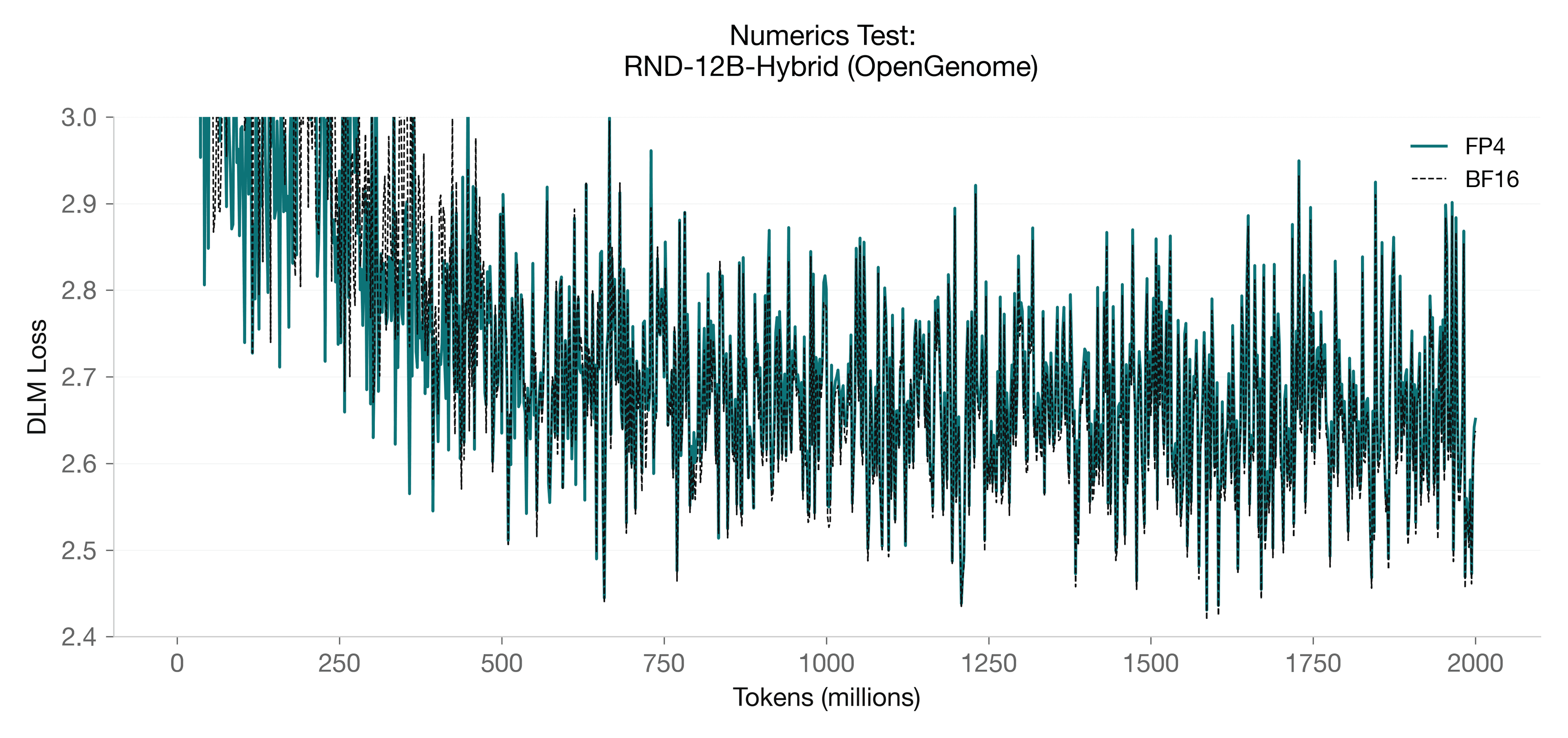
Challenges in scaling on long DNA sequences helped drive our early long-context work (Hyena, HyenaDNA), culminating in Evo. But bridging the gap going forward will not be the result of model architecture breakthroughs alone. Instead, it requires co-developing training objectives, architectures and scaling recipes. For example, a new hybrid architecture trained with discrete diffusion objectives will induce activation and gradient distributions which may be better suited to a different mixture of numeric data types, compared to a more classical autoregressive model.
This post is the first in a series dedicated to low-precision pretraining, starting with NVIDIA's NVFP4 pretraining recipe. We cover the theory, supported with self-contained PyTorch examples to ground concepts, then dive into the weeds of NVIDIA's official implementation, dissecting the systems optimizations and fused kernels to make NVFP4 training performant.
In this series:
- (This post) – Mixed precision background, the
NVFP4recipe, and the theory behind each technique - Part 2: Systems Optimizations – Systems optimizations and custom kernels for making
NVFP4performant - (Future) Ablations and insights on pretraining custom hybrid architectures under
MXformats - (Future) Custom recipes and kernels for improved
MXmixed-precision
Why FP4 Training?
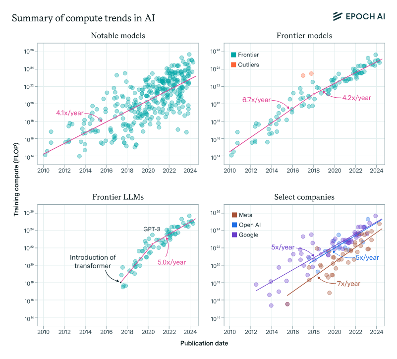
Training compute for frontier LLMs is growing at a rate of 4-5x / year.
4th generation tensor cores enabled FP8 mixed precision training, boosting throughput ~1.5-2.0x relative to FP16 with minimal loss of quality. The ever-increasing demand for compute, however, continues the push for smaller data formats and more FLOPs.
With the formalization of microformats and hardware support with 5th generation tensor cores, narrow-precision training with FP4 is now possible, with a 4x increase in throughput over FP16 tensor cores.
However, training at such limited bitwidth requires specialized protocols as we are nearing the limits of range and precision.
Implementing these techniques while preserving performance requires a combination of numerical methods and careful systems engineering.
Starting Point: NVFP4 Recipe at a Glance
NVIDIA's recipe achieves numerical stability through four complementary techniques:
| Technique | Target Problem | Applied To |
|---|---|---|
| Random Hadamard Transform | Activation outliers | Wgrad inputs |
| Stochastic Rounding | Gradient bias | Gradients |
| 2D Block Scaling | Chain-rule violation | Weights |
| Selective Precision | Sensitive layers | Last ~15% of layers |
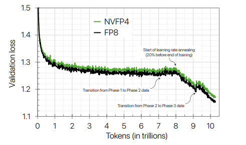
We start our discussion with NVIDIA's NVFP4 recipe given that it has been validated at scale (12B hybrid model trained to 10T tokens).
While there have been many alternatives proposed that might be more theoretically thorough, the NVIDIA recipe has a production-level implementation to back extensive ablations so is a safe base from which to start the discussion.
We will discuss exploration and experimentation with alternative protocols in future blogposts.
Background: Floating Point Fundamentals
Before diving into narrow-precision training, let's establish the core concepts that govern how floating point formats represent real numbers.
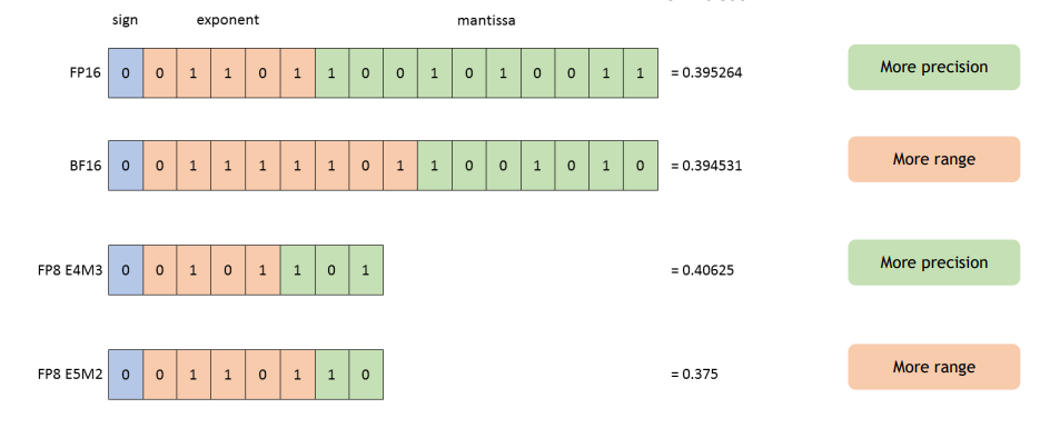
The IEEE 754 Encoding
A floating point number is encoded as three fields:
| Field | Purpose |
|---|---|
| Sign (S) | |
| Exponent (E) | Dynamic range |
| bias | Offset calculated at , where is the number of exponent bits for a specific floating point format |
| Mantissa (M) | Fractional precision |
The exponent determines dynamic range, or how many orders of magnitude can be represented. The mantissa determines precision, or how many samples exist between consecutive powers of 2.
The floating point formula above is for normals, where and .
IEEE defines the following special cases:
- : zero and sub-normals
- : normals
- : Inf/NaN
where is the number of exponential bits for a specific floating point format.
For sub-normals, the formula is:
Briefly, the reason for sub-normals is to allow for gradual underflow, allowing smoother transition from the smallest normal () down to in mantissa () gradations, where m is the number of mantissa bits for a specific floating point format.
As an example, the min sub-normal and max normal for FP8_E4M3 can be calculated as so:
# FP8_E4M3
e = 4  # exponent bits
m = 3  # mantissa bits
bias = 2 ** (e - 1) - 1

# Min subnormal encoding
sign = 0
e_bits = 0b0000      # exponent = 0 signals subnormal
m_bits = 0b001       # smallest non-zero mantissa

E_debiased = 1 - bias
M = m_bits / (2 ** m)

min_subnormal = (-1) ** sign * (2 ** E_debiased) * M
Sign: 0
Exponent bits: 0000 = 0
Mantissa bits: 001 = 1
Bias = 2^(4-1) - 1 = 2^3 - 1 = 7
Debiased exponent = 1 - bias = 1 - 7 = -6
Mantissa value = 1/8 = 0.125 (No implied 1 for subnormals)

Min subnormal = 2^-6 × 0.125
      = 0.015625 × 0.125
      = 0.001953125
# Max normal
sign = 0
# Note: 0b11111111 is reserved for NaN
e_bits = 0b1111    # largest exponent
m_bits = 0b110     # largest mantissa

E_debiased = (e_bits - bias)
M = m_bits / (2 ** m)

max_normal = (-1) ** sign * (2 ** E_debiased) * (1 + M)
Sign: 0
Exponent bits: 1111 = 15
Mantissa bits: 110 = 6
Max normal = 2^8 × 1.75
      = 256 × 1.75
      = 448.0
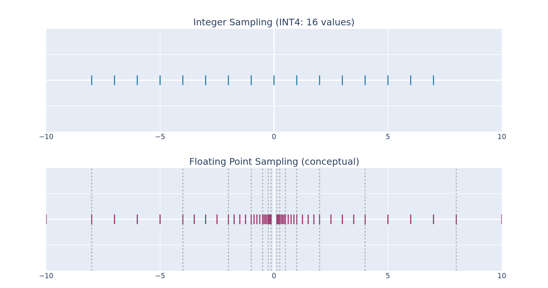
Sampling the Real Number Line
Unlike integers, which sample uniformly, floating point numbers sample logarithmically, with equal density between each pair of consecutive powers of 2.
Dynamic Range: Binades
A binade is one power of 2 of dynamic range.
The dynamic range of a format:
| Format | Exponent Bits | Binades | Implication |
|---|---|---|---|
| FP32 | 8 | ~277 | Sufficient for most computations |
| FP16 | 5 | ~40 | Sufficient for most activations |
| BF16 | 8 | ~261 | FP32 range, limited precision |
| FP8 E4M3 | 4 | ~18 | Suitable for FP8 training fwd pass |
| FP8 E5M2 | 5 | ~32 | Needed for FP8 training bwd pass |
| FP4 E2M1 | 2 | ~3.6 | Very constrained |
FP4's 3.6 binades cannot represent typical tensor value distributions, which often span 10-20 binades. This is why block scaling becomes essential.
The Evolution of Mixed-Precision Training
FP16 Mixed Precision (2017)
The original mixed-precision recipe was motivated by the introduction of FP16 tensor cores, which can provide substantially higher throughput than FP32 for supported GEMMs/convolutions.
In the recipe, an FP32 master copy of the weights is maintained for the optimizer update, while forward and backward computation uses FP16. To mitigate FP16 gradient underflow, loss scaling is used, where the loss is multiplied by a scale factor before backpropagation, and gradients are unscaled (divided by the same factor) before the optimizer step. With dynamic loss scaling, the scale is adjusted based on overflow detection; when overflow is detected, the optimizer step is typically skipped and the scale is reduced.
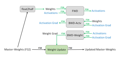
More recent FP16 mixed precision training has shifted towards bfloat16, which removes the need for a scaling factor given this dtype's greater dynamic range.
FP8 Mixed Precision (2022)
FP8 training, formalized by Micikevicius et al. (2022), became feasible at scale with the introduction of FP8 tensor cores.
Notable differences from the original mixed precision recipe are the use of different formats for forward / backward, per-tensor scaling, and different scaling recipes.
Dual formats: E4M3 vs E5M2
| Format | Exponent | Mantissa | Max Value | Use Case |
|---|---|---|---|---|
| E4M3 | 4 | 3 | 448 | Forward pass (precision) |
| E5M2 | 5 | 2 | 57344 | Backward pass (range) |
Per-tensor scaling
Given the limited range of FP8 relative to FP16 formats, per-tensor (or even finer-grained) scale factors are needed to shift the tensor distributions within the representable range.
Scaling Recipes
There are various ways to implement FP8 mixed precision:
-
Per Tensor
- Delayed Scaling: Rather than computing scale factors on-the-fly, FP8 training maintains an amax history and computes scales from historical maxima. This amortizes the cost of scale computation but requires maintaining and tuning the history window to retain accuracy.
- Current Scaling: There is also current scaling, where the
amaxis calculated on-demand, trading performance for potentially greater accuracy than delayed scaling.
-
Per-channel: Finer grained scaling, such as per-row is possible as well, again with greater accuracy but higher overhead than delayed and current scaling .
-
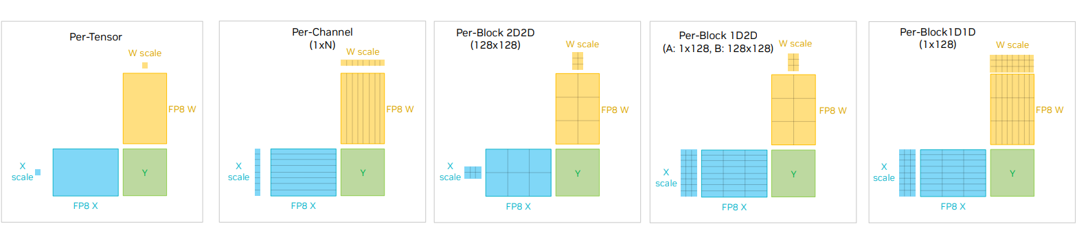
Per-block: The Deepseek-v3 team was one of the first to demonstrate the feasibility of blockwise quantization without hardware support, as detailed in Deepseek et al. (2024). They used
128 x 1blocks for activations and gradients, and128 x 128blocks for weights, along with some additional hardware tricks to mitigate low-precision numerical instabilities.
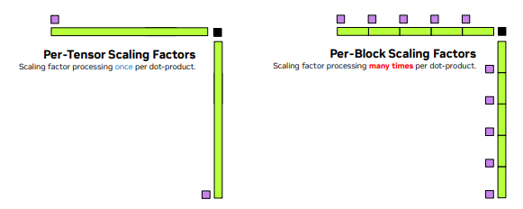
The figure below illustrates various FP8 scaling strategies, from per-tensor to blockwise, each a different point along the throughput / accuracy spectrum.
Microscaling and MX formats
The microscaling paradigm shifts from per-tensor to per-block scaling.
Microscaling formats push scaling into the datatype itself:
- Store data in a narrow element format (FP8/FP6/FP4).
- Store per-block metadata (an 8-bit scale factor) to recover range.
- 5th gen tensor cores natively consume data and metadata.
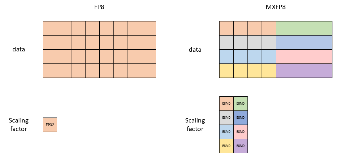
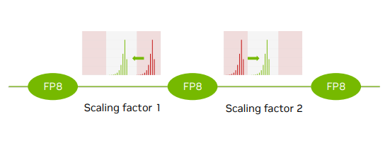
The key idea is that even though 10-20 binades might be needed to represent entire tensors, the dynamic range within blocks of a tensor is within the representable range of FP8E4M3.
Since each block is quantized independently with its own scale factor, the per-block distributions can be shifted and compressed into the requisite range.
The tradeoff – without native hardware support – is performance: since the block size (32) is typically much smaller than the reduction dimension K, each block needs to be scaled within the GEMM mainloop.
When scale factors are per-tensor or per-row, the scaling can be folded into the epilogue of the GEMM, whereas per-block scaling requires software intervention within the accumulation mainloop of the GEMM.
With Blackwell 5th generation tensor cores, this scaling is directly handled by hardware.
Main takeaways from blockwise scaling:
-
Localize the impact of outliers: in per-tensor scaling, a single outlier compresses all values. With block scaling, outliers only affect their local block.
-
Increased accuracy: By using multiple scale factors per tensor, we can shift the observed range within each block so that it fits within the dynamic range of
FP8. This allows for the use ofE4M3as the storage format, whereas in the traditional per-tensorFP8recipe, a hybrid strategy ofE4M3was needed for the forwards pass andE5M2for the backward pass.
MXFP8 Specification
| Component | MXFP8 |
|---|---|
| Data format | E4M3 |
| Block size | 32 elements |
| Scale format | E8M0 |
The UE8M0 scale format uses all 8 bits for exponent with no mantissa, giving 256 power-of-two scales.
Additionally, the OCP specs define microformats for FP6 (E{2,3}M{3,2}) and FP4 (E2M1) with the same block size and scale format as MXFP8.
The Transpose Problem
Block scaling introduces a subtle issue for training. Since block scaling is along reduction dimension K, a quantized tensor and its quantized transpose are no longer equivalent.
Specifically,
- Forward: -> scales along rows of
- Backward (Wgrad): -> scales along columns of
From an implementation standpoint, this requires performing the quantization of a tensor and its transpose during the same pass to prevent double quantization errors.
From a mathematical standpoint, this introduces issues with chain-rule consistency, since the inputs to the forward and backward passes are no longer equivalent, as we'll see in upcoming sections.
Two-Level Scaling for 4-Bit Training
The NVFP4 Format
NVFP4 extends microscaling to 4 bits with a two-level scaling scheme.
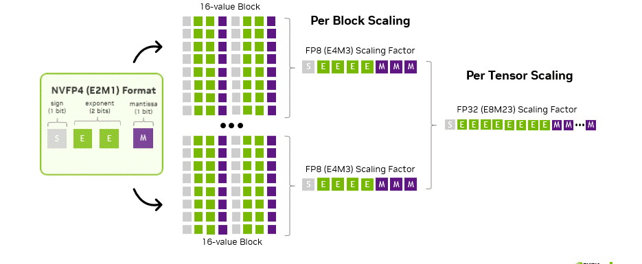
Why Two Levels?
With only 3.6 binades of FP4 dynamic range and 1 bit of mantissa, block-level scales in FP8 E4M3 are needed for scale-factor precision.
A second FP32 global scale factor is then used to mitigate overflow given the limited range of E4M3.
More concretely:
- The global encode scale remaps values so the largest value in the tensor is within the representable product range of (FP4 max) × (FP8 E4M3 max).
- Local decode scales are computed per block, quantized to
E4M3by using global encode scale, then inverted to get back a usable local encode scale.
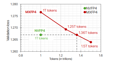
This is in contrast to MXFP4, the official OCP FP4 microformat:
MXFP4has a singleE8M0blockwise scale factorE8M0has the full dynamic range ofFP32, but this increased range comes at the cost of precisionMXFP4also uses a larger block size:32vs16
Despite the greater range of the scale factor, the reduced precision makes it a less stable format for pre-training.
Training with MXFP4 is feasible, however: it requires either more tokens to reach the same loss as NVFP4 as shown by NVIDIA et al (2025) or alternative recipes per Castro et al (2025).
NVFP4 Quantization Protocol
For a tensor with blocks :
-
Compute global amax (
FP32): -
Compute global encode / decode scales (
FP32): ,
where 6.0 and 448.0 are the largest E2M1 and E4M3 normals, respectively.
-
Compute blockwise decode scales in original high precision dtype (
BF16/FP16/FP32) then cast toFP32:
where is the local absmax within a 1 x 16 block.
-
Quantize (
RTNE) blockwise scales toFP8E4M3: -
Calculate the "correct" blockwise encoding factors:
-
Quantize (
RTNEor stochastic round) high precision values toFP4E2M1:
Note that the recipe does not use the original blockwise scales to quantize values to FP4E2M1.
- Scales are first quantized to
FPE4M3then upcast toFP32before using forFP4E2M1encoding. - This is so that the roundtrip conversion and the original values can be recovered.
Tensor-level scaling means you (naively) need:
- one pass to compute tensor amax,
- another pass to apply the global scale before block quantization.
This is an extra round-trip through memory and matters at scale.
We will see in Part 2: Systems Optimizations how frameworks such as TransformerEngine implement these additional ops in a performant manner.
The following code emulates this quantization procedure in PyTorch:
import torch
import numpy as np

# FP4 E2M1 constants
FLOAT4_E2M1_MAX = 6.0
FLOAT8_E4M3_MAX = 448.0
FLOAT32_MAX = torch.tensor(torch.finfo(torch.float32).max, dtype=torch.float32)
NVFP4_BLOCKSIZE = 16

def blockwise_quantize_nvfp4(x: torch.Tensor, tile_shape: list = [1, NVFP4_BLOCKSIZE]):
    """Quantize tensor to NVFP4 format with blockwise scaling."""
    M, N = x.shape
    tile_y, tile_x = tile_shape

    # Global amax and scales
    global_amax = torch.amax(torch.abs(x))
    global_encode_scale = torch.div(FLOAT8_E4M3_MAX * FLOAT4_E2M1_MAX, global_amax)
    global_encode_scale = torch.min(global_encode_scale, FLOAT32_MAX)
    if global_encode_scale == 0.0:
        global_encode_scale = torch.tensor(1.0, dtype=torch.float32)
    global_decode_scale = torch.div(1.0, global_encode_scale)

    # Blockwise scales
    x_reshaped = x.view(M, N // tile_x, tile_x)
    blockwise_amax = torch.amax(torch.abs(x_reshaped), dim=-1, keepdim=True).to(torch.float32)
    decode_scales = torch.div(blockwise_amax, FLOAT4_E2M1_MAX)
    decode_scales = decode_scales * global_encode_scale
    decode_scales = torch.clamp(decode_scales, min=-FLOAT8_E4M3_MAX, max=FLOAT8_E4M3_MAX)
    decode_scales = decode_scales.to(torch.float8_e4m3fn)

    encode_scales = torch.div(1.0, decode_scales.to(torch.float32) * global_decode_scale)
    encode_scales = torch.min(encode_scales, FLOAT32_MAX)

    # Scale input
    x = x.view(M, N // tile_x, tile_x)
    scaled_x = x.to(torch.float32) * encode_scales
    scaled_x = torch.clamp(scaled_x, -FLOAT4_E2M1_MAX, FLOAT4_E2M1_MAX).reshape(M, N)

    return scaled_x, encode_scales, decode_scales, global_amax

def round_to_nearest_even(x: torch.Tensor):
    """Round to nearest FP4 E2M1 value using round-to-nearest-even."""
    result = torch.zeros_like(x, dtype=torch.float32)

    # Positive values
    result[(x >= 0.0) & (x <= 0.25)] = 0.0
    result[(x > 0.25) & (x < 0.75)] = 0.5
    result[(x >= 0.75) & (x <= 1.25)] = 1.0
    result[(x > 1.25) & (x < 1.75)] = 1.5
    result[(x >= 1.75) & (x <= 2.5)] = 2.0
    result[(x > 2.5) & (x < 3.5)] = 3.0
    result[(x >= 3.5) & (x <= 5.0)] = 4.0
    result[x > 5.0] = 6.0

    # Negative values
    result[(x >= -0.25) & (x < -0.0)] = -0.0
    result[(x < -0.25) & (x > -0.75)] = -0.5
    result[(x <= -0.75) & (x >= -1.25)] = -1.0
    result[(x < -1.25) & (x > -1.75)] = -1.5
    result[(x <= -1.75) & (x >= -2.5)] = -2.0
    result[(x < -2.5) & (x > -3.5)] = -3.0
    result[(x <= -3.5) & (x >= -5.0)] = -4.0
    result[x < -5.0] = -6.0

    return result

def dequantize_fp4(qx, decode_scales, global_amax, tile_shape=[1, NVFP4_BLOCKSIZE]):
    """Dequantize from FP4 E2M1 back to FP32."""
    tile_y, tile_x = tile_shape
    M, N = qx.shape
    global_decode_scale = global_amax / (FLOAT4_E2M1_MAX * FLOAT8_E4M3_MAX)
    decoded_block_scales = decode_scales.to(torch.float32) * global_decode_scale
    qx = qx.view(M, N // tile_x, tile_x)
    if decoded_block_scales.ndim == 2:
        decoded_block_scales = decoded_block_scales.unsqueeze(-1)
    return (qx * decoded_block_scales).reshape(M, N)
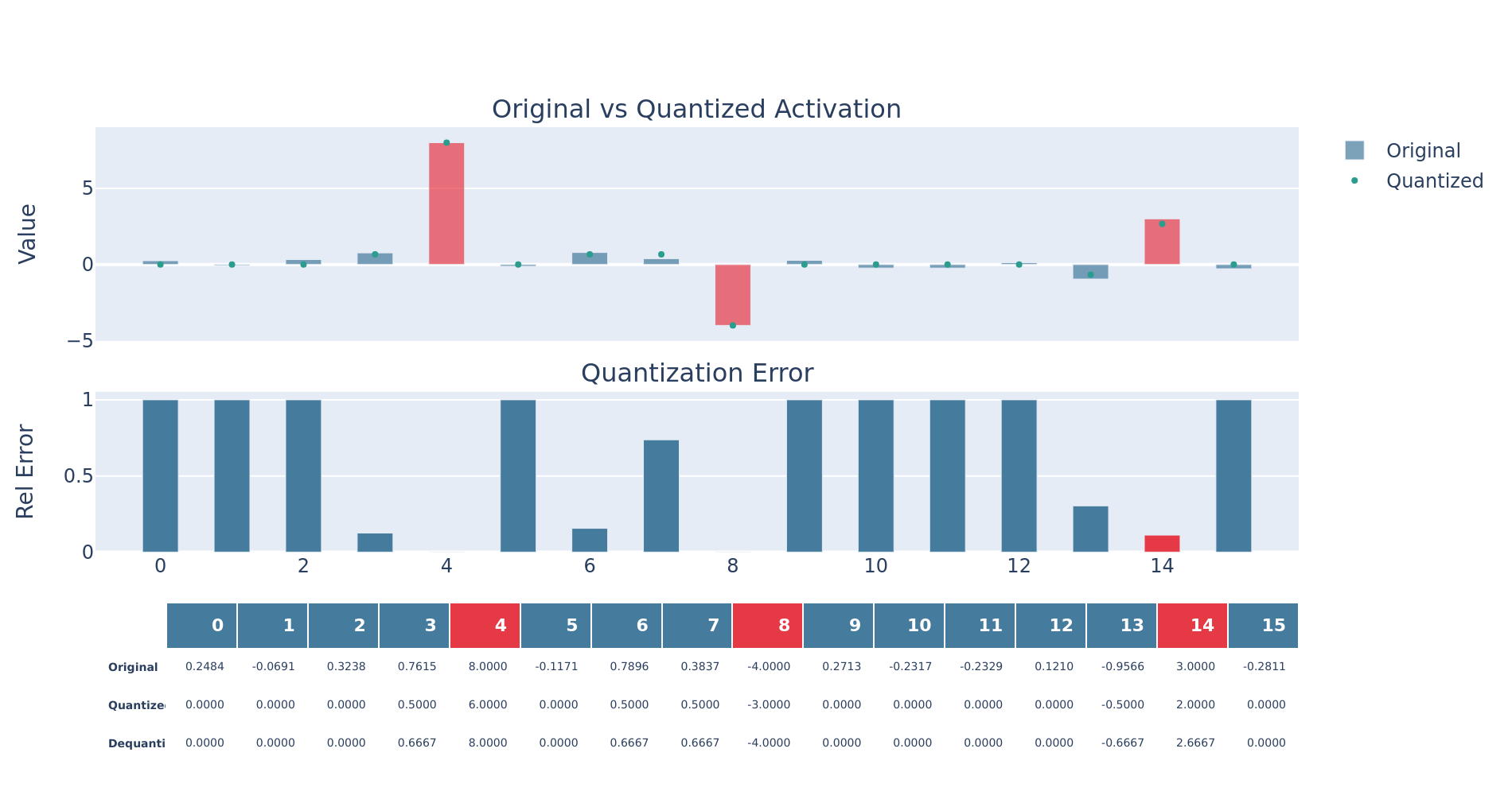
Running blockwise quant for a single 1 x 16 tensor:
x = torch.tensor(
    [0.0, 0.25, 0.5, 0.75356, 1.251245, 3.2002, 4.5032, 15.011, 0.012, -0.312, -5.50055, 10.06, -1.2526, 3.025, 2.5114, 7.0162]
)

scaled_x, encode_scales, decode_scales, global_amax = blockwise_quantize_nvfp4(x.unsqueeze(0))
qx = round_to_nearest_even(scaled_x)
dq = dequantize_fp4(qx, decode_scales, global_amax)
| Input (FP32) | FP4 Domain | Dequantized (FP32) | |
|---|---|---|---|
| Scaled | Quantized | ||
| 0.0000 | 0.0000 | 0.0000 | 0.0000 |
| 0.2500 | 0.0999 | 0.0000 | 0.0000 |
| 0.5000 | 0.1999 | 0.0000 | 0.0000 |
| 0.7536 | 0.3012 | 0.5000 | 1.2509 |
| 1.2512 | 0.5001 | 0.5000 | 1.2509 |
| 3.2002 | 1.2791 | 1.5000 | 3.7528 |
| 4.5032 | 1.7998 | 2.0000 | 5.0037 |
| 15.0110 | 6.0000 | 6.0000 | 15.0110 |
| 0.0120 | 0.0048 | 0.0000 | 0.0000 |
| −0.3120 | −0.1247 | 0.0000 | 0.0000 |
| −5.5005 | −2.1986 | −2.0000 | −5.0037 |
| 10.0600 | 4.0211 | 4.0000 | 10.0073 |
| −1.2526 | −0.5007 | −0.5000 | −1.2509 |
| 3.0250 | 1.2091 | 1.0000 | 2.5018 |
| 2.5114 | 1.0038 | 1.0000 | 2.5018 |
| 7.0162 | 2.8044 | 3.0000 | 7.5055 |
| Encode scales: 0.3997 (single blockwise scale factor in this case) | |||
| Global amax: 15.0110 |
NVFP4 Blockwise GEMM
As discussed earlier, blockwise GEMM requires hardware support to be computationally efficient.
To see why, we can emulate a blockwise GEMM in pure PyTorch:
import torch

FLOAT4_E2M1_MAX = 6.0
FLOAT8_E4M3_MAX = 448.0
NVFP4_BLOCKSIZE = 16

FP4_VALUES = torch.tensor(
    [
        0.0,  # 0000
        0.5,  # 0001
        1.0,  # 0010
        1.5,  # 0011
        2.0,  # 0100
        3.0,  # 0101
        4.0,  # 0110
        6.0,  # 0111
        -0.0, # 1000
        -0.5, # 1001
        -1.0, # 1010
        -1.5, # 1011
        -2.0, # 1100
        -3.0, # 1101
        -4.0, # 1110
        -6.0, # 1111
    ],
    dtype=torch.float32,
)

def cast_from_fp4(qx, out_dtype) -> torch.Tensor:
    return FP4_VALUES[qx.to(torch.long)].to(out_dtype)

def gemm(
    A: torch.Tensor,
    B: torch.Tensor,
    out_dtype: torch.dtype = torch.float32,
) -> torch.Tensor:
    A = A.to(out_dtype)
    B = B.to(out_dtype)
    return A @ B

# Adapted from TransformerEngine: https://github.com/NVIDIA/TransformerEngine/blob/2f8ae81c3b78db38f5ace8735eedb66269159c91/transformer_engine/pytorch/custom_recipes/quantization_nvfp4.py#L771-L887
def blockwise_quantized_gemm_ref(
    qx: torch.Tensor,
    qw: torch.Tensor,
    sx: torch.Tensor,
    sw: torch.Tensor,
    global_amax_x: torch.Tensor,
    global_amax_w: torch.Tensor,
    out_dtype: torch.dtype = torch.float32
) -> torch.Tensor:
    """Python emulation of blockwise FP4 GEMM.

    qx: float4_e2m1 tensor
    qw: float4_e2m1 tensor
    sx: float8_e4m3 scale factors
    sw: float8_e4m3 scale factors
    global_amax_x: float32 global scale factor
    global_amax_w: float32 global scale factor
    """
    # Convert from encoded fp4 to equivalent fp32 value
    x = cast_from_fp4(qx, out_dtype)
    w = cast_from_fp4(qw, out_dtype)

    # Direct cast from fp8_e4m3 -> fp32
    sx = sx.to(torch.float32)
    sw = sw.to(torch.float32)

    # Calculate global decode scale factors
    MAX_NORMS_SQ = FLOAT4_E2M1_MAX * FLOAT4_E2M1_MAX * FLOAT8_E4M3_MAX * FLOAT8_E4M3_MAX
    alpha = torch.div(global_amax_x * global_amax_w, MAX_NORMS_SQ).squeeze(-1)

    M, K = x.shape
    N, K_w = w.shape
    assert K == K_w, "K dimension mismatch between qx and qw"

    grid_k = K // NVFP4_BLOCKSIZE

    y = torch.zeros(M, N, dtype=torch.float32, device=qx.device)

    # Emulates FP4 tensor core implementation
    # Each output element (i, j) is fp32 accumulation of (K // block_length) inner products
    for k in range(grid_k):
        k_start = k * NVFP4_BLOCKSIZE
        k_end = k_start + NVFP4_BLOCKSIZE

        qx_block = x[:, k_start:k_end].clone().contiguous()
        qw_block = w[:, k_start:k_end].clone().contiguous()

        # Extract scaling factors for the current blocks
        sx_block = sx[:, k]
        sw_block = sw[:, k]

        y += torch.outer(sx_block, sw_block) * gemm(qx_block, qw_block.T, torch.float32)

    y = alpha * y
    y = y.to(out_dtype)
    return y
Contrast this with the conventional triply nested GEMM, which can be efficiently parallelized and vectorized: the problem is the per-block scaling, which interrupts the GEMM mainloop and can not be folded into the epilogue.
NVFP4 vs MXFP4 vs MXFP8
| Feature | MXFP8 | MXFP4 | NVFP4 |
|---|---|---|---|
| Data format | E4M3 | E2M1 | E2M1 |
| Block size | 32 | 32 | 16 |
| Scale format | E8M0 | E8M0 | E4M3 |
| Scale levels | 1 | 1 | 2 (block + global) |
The NVFP4 Recipe
The recipe presented in Pretraining Large Language Models with NVFP4 called out 4 techniques for stabilizing NVFP4 training:
- Random Hadamard Transforms
- Stochastic Rounding
- 1D / 2D Blockscaling
- Selective Precision
Random Hadamard Transforms (RHT)
LLM activations exhibit heavy-tailed distributions, where a few channels contain values orders of magnitude larger than the median. When quantizing to FP4, the outliers force a large scale factor, causing underflow and ineffective use of the already limited range.
The Hadamard transform redistributes outliers, transforming heavy-tailed distributions to Gaussian-like and more conducive to quantization.
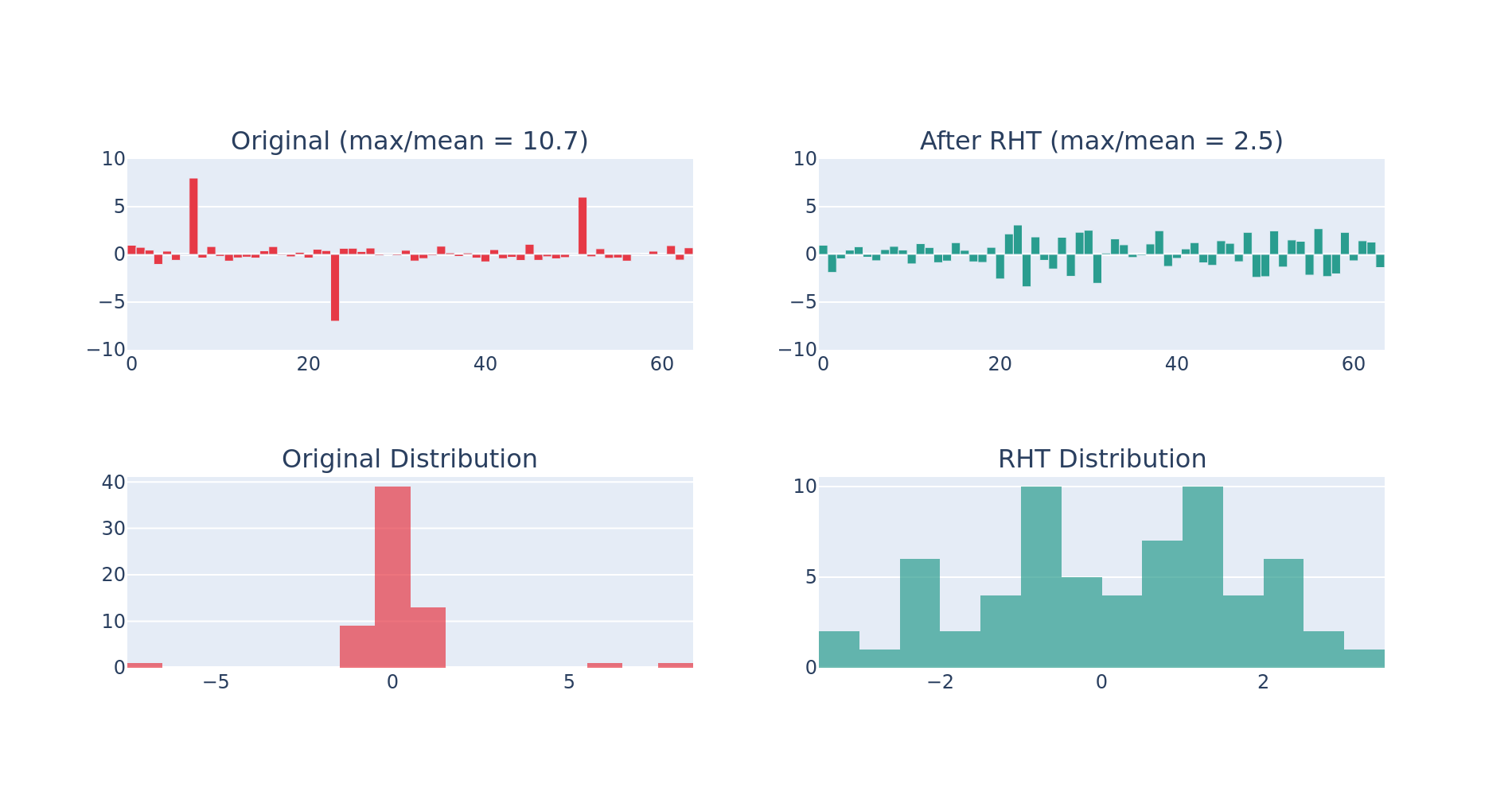
# Toy Experiment to demonstrate effects of Hadamard Transform

import torch

torch.manual_seed(42)

n = 64
x = torch.randn(n) * 0.5
x[7] = 8.0   # Outlier
x[23] = -7.0  # Outlier
x[51] = 6.0   # Outlier

# Apply RHT
H = build_hadamard_matrix(n)
x_ht = x @ H

# Statistics
def compute_stats(tensor):
    return {
        'max': tensor.abs().max().item(),
        'mean': tensor.abs().mean().item(),
        'max/mean': (tensor.abs().max() / tensor.abs().mean()).item(),
        'std': tensor.std().item()
    }

stats_orig = compute_stats(x)
stats_ht = compute_stats(x_ht)
| Metric | Original | After HT |
|---|---|---|
| max | 8.000 | 3.397 |
| mean | 0.745 | 1.385 |
| max/mean | 10.732 | 2.452 |
| std | 1.615 | 1.615 |
Using the max/mean ratio as a rough proxy for outlier impact, we can see that that this ratio drops after applying the Hadamard transform.
Orthogonal Mixing as a Quantization Preconditioner
FP4 quantization (especially with a single scale per block) is basis-dependent: the same vector can be easy or hard to quantize depending on which coordinates carry the energy. If a few channels dominate, they set the scale and everyone else underflows.
An orthogonal change of basis lets us "rotate" the channels without changing the exact math of the GEMM (as long as the same is applied on both sides of the inner dimension):
We can pick to make activations (and weights) more isotropic within each quantization group: lower mean and fewer extreme values per coordinate. What makes a good ?
- Strong mixing. A clean way to measure "outlier spread" is coherence . The theoretical minimum is , achieved when all entries have magnitude . Hadamard matrices achieve this minimum exactly.
- Fast + hardware-friendly. structure (butterflies) or a form that maps well to fused kernels.
- Easy inverse. For orthogonal transforms, , no extra conditioning required.
There are a few canonical transforms of this class:
| Transform | Pros | Cons |
|---|---|---|
| Hadamard | Minimum coherence and very fast | Fixed structure can have rare unlucky alignments |
| Randomized Hadamard | Hadamard + avoids worst-case alignment | Small overhead for RNG/sign storage |
| DCT / FFT-like bases | High compression for signals with structured spectrum | Less uniform mixing; FFT can introduce complex ops/constants |
| Dense random orthogonal | Excellent mixing | cost |
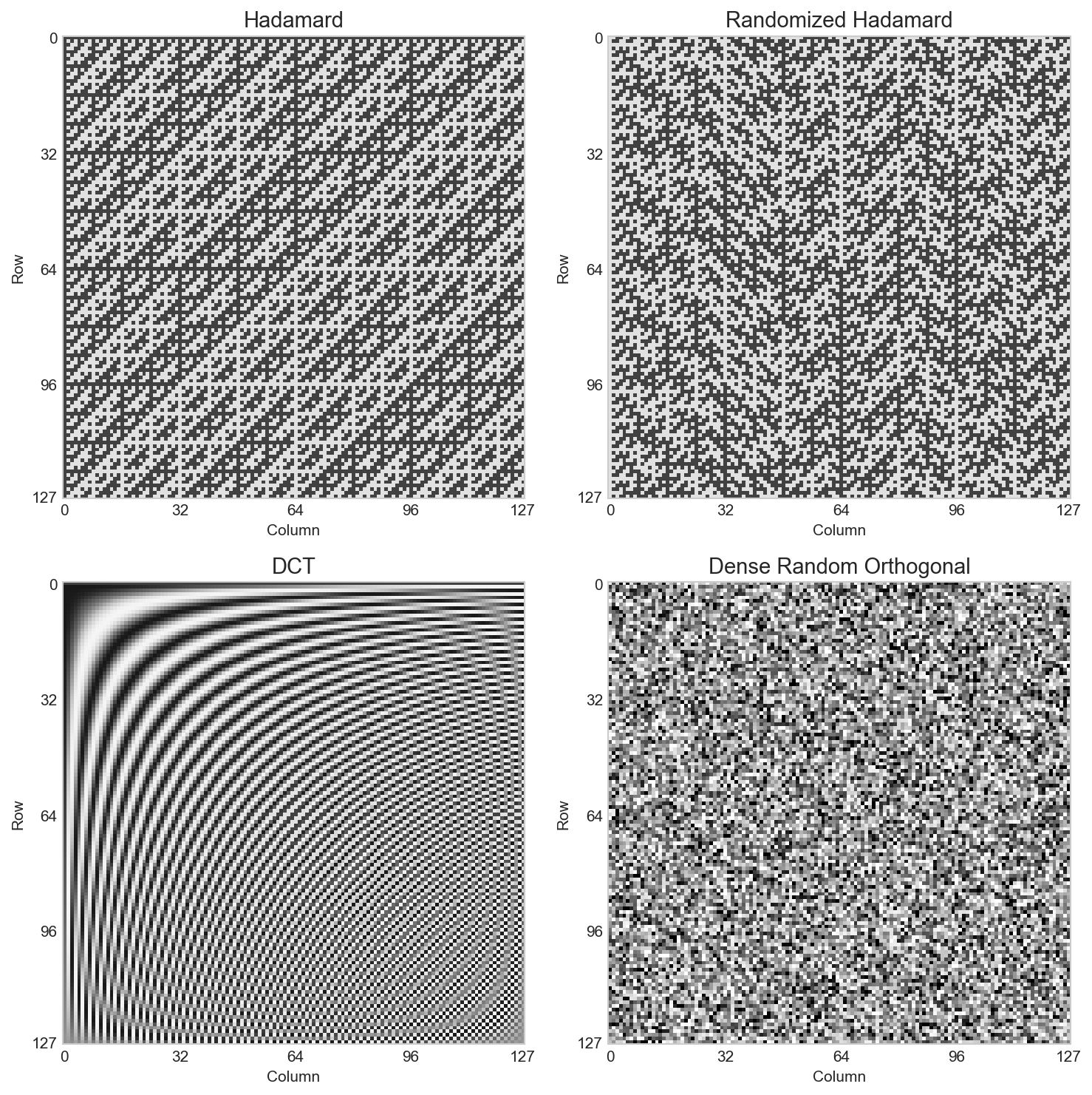
A Hadamard matrix is an orthogonal matrix with entries where is a power of 2.
import torch

def build_hadamard_matrix(n: int, dtype: torch.dtype = torch.float32) -> torch.Tensor:
    """Generate n×n Hadamard matrix (n must be power of 2)"""
    assert n > 0 and (n & (n-1)) == 0, "n must be a power of 2"

    if n == 1:
        return torch.tensor([[1.0]], dtype=dtype)

    H_half = build_hadamard_matrix(n // 2)
    H = torch.cat([
        torch.cat([H_half, H_half], dim=1),
        torch.cat([H_half, -H_half], dim=1)
    ], dim=0) / (2 ** 0.5)

    return H
Note that the recipe uses a randomized Hadamard matrix:
- The standard Hadamard matrix has fixed structure.
- If outliers happen to align with Hadamard basis vectors, they won't be effectively redistributed.
The randomized version adds a random sign flip:
where is a random sign vector.
def get_wgrad_sign_vector(n: int, dtype: torch.dtype = torch.float32) -> torch.Tensor:
    v = torch.randint(0, 2, (n,), dtype=torch.int8) * 2 - 1  # values in {-1, +1}
    return v.to(dtype)

def apply_rht(n: int, dtype: torch.dtype = torch.float32, randomize: bool = False) -> torch.Tensor:
    """Construct randomized hadamard matrix"""
    H = build_hadamard_matrix(n, dtype)
    if randomize:
        sign_mat = get_wgrad_sign_vector(n, dtype) * torch.eye(n, dtype=dtype)
        H = sign_mat @ H

    return H
In NVIDIA's recipe, a single random sign vector is hardcoded. This ensures consistent transforms without per-layer overhead without any downstream pathologies.
Where RHT is Applied in the NVFP4 Recipe
RHT is applied only to Wgrad inputs, as experimental results showed no benefit to applying to FProp and DGrad inputs.
Moreover, an RHT of size 16 x 16 was chosen to balance accuracy and performance: too small and accuracy suffers due to insufficient redistribution of outliers; too large and the computation and memory costs become too expensive.
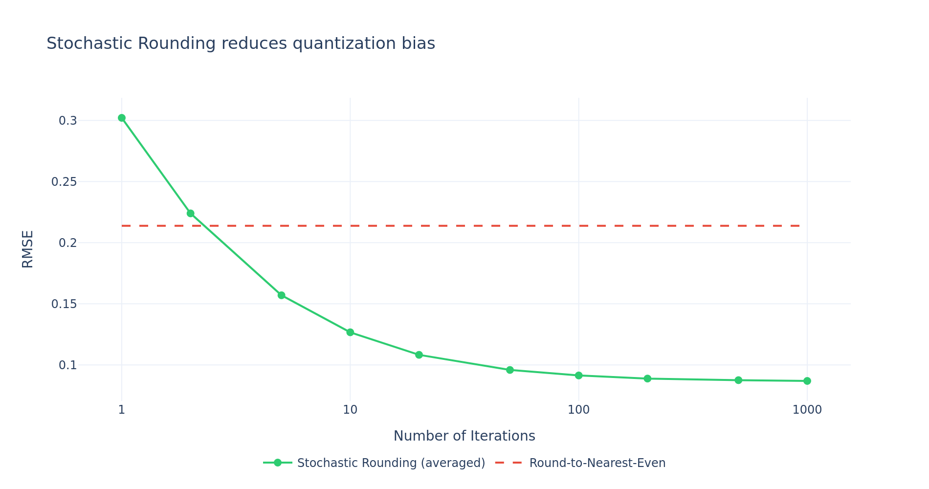
Stochastic Rounding (SR)
During quantization to FP4, rounding using RTNE (round-to-nearest-even) can introduce systematic biases, leading to values always being quantized in a certain direction. NVIDIA observed that the bias from deterministic rounding had a pronounced effect on gradients which led to training instability.
The solution is stochastic rounding:
- Values are probabilistically rounded to the two nearest representation levels, with probabilities inversely proportional to distance:
- This reduces bias at the cost of greater variance.
# FP4 E2M1 representable values
FP4_E2M1_VALS = torch.tensor([
    0.0, 0.5, 1.0, 1.5, 2.0, 3.0, 4.0, 6.0,  # Positives
    -0.0, -0.5, -1.0, -1.5, -2.0, -3.0, -4.0, -6.0,  # Negatives
], dtype=torch.float32)

def stochastic_round(x: torch.Tensor):
    """Stochastically round to FP4 E2M1 values based on proximity.
    Args:
        x: tensor with values scaled **and** clamped to lie within the FP4 range
        but not yet rounded to FP4 values.
    """

    # 1. Calculate distance to nearest FP4 vals
    dist = x.view(-1, 1).sub(FP4_E2M1_VALS.unsqueeze(0)).abs()
    # 2. Take 2 closest FP4 levels
    nearest_dist, nearest_idx = dist.topk(k=2, dim=-1, largest=False)
    fp4_neighbors = FP4_E2M1_VALS[nearest_idx.view(-1).to(torch.long)].reshape(-1, 2)

    # 3. Denominator for prob calculation is the distance between closest FP4 levels
    den = fp4_neighbors.diff().abs()
    den = torch.where(den == 0.0, 1.0, den)

    # 4. Smaller distance -> Higher prob
    prob = (1 - (nearest_dist / den)).abs()

    # 5. Probabilistically select based on distance
    select_idx = nearest_idx.gather(1, torch.multinomial(prob, 1).view(-1).to(torch.long).unsqueeze(-1))

    # 6. Finally return the actual FP4 vals selected
    return FP4_E2M1_VALS[select_idx.view(-1)].reshape(x.shape)
SR in the NVFP4 Recipe
It was observed that the gradients are particularly sensitive to quantization bias while there was no benefit to applying SR to other tensors, and in fact could harm convergence when applied in FProp by amplifying quantization errors relative to RTNE.
1D vs 2D Block Scaling
The Chain Rule Problem
In the forward pass GEMM FProp, and are quantized rowwise, while in the backward pass GEMMs, quantization orientations are flipped, e.g. and .
Specifically, with 1D block scaling, since blockwise quantization is always along the reduction dimension. This violates the chain rule, which requires the same inputs for the forward and backprop.
To address this issue, 2D 16 x 16 blocks are used when quantizing weights to preserve symmetry; 1D 1 x 16 are used for other tensors.
Technically, activations and gradient tensors also violate the chain rule given the asymmetry of quantization in forward prop and backprop:
- → and are quantized along rows
- → and are quantized along columns
- → and are quantized along rows
NVIDIA et al (2025) observed that:
- Activations and gradients benefit more from the increased quantization of finer-grained scaling (1D
1 x 16blocks) - Weights are less sensitive to coarser-grained quantization and are able to adapt to the quantization range.
Moreover, they performed ablations using various combinations of block quantization:
1 x 16scaling along the same dimension for both forward and backward – consistent representation, no chain rule violation1 x 16scaling along different dimensions for forward / backward – inconsistent, violates chain rule, but practically necessary16 x 16scaling – consistent
Only the 2nd and 3rd options are actually feasible, again because of tensor core requirements.

To summarize:
- Weights:
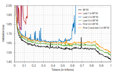
1 x 16scaling along the same dimension hews closest to the reference loss but is not feasible due to hardware constraints.16 x 16block scales are a compromise between consistency and accuracy. - Activations: Less sensitive to chain-rule inconsistency and effects show only in the later stages of training (during weight decay under a WSD schedule) which can be mitigated by switching to higher precision for the cooldown phase.
Selective Precision
Operator Selection
Linear layers are usually the first to be quantized, while other operators are kept in higher precision.
Layer Selection
Empirical analysis showed that first and last layers are more sensitive to quantization error.
Notably, the authors of the NVFP4 paper observed that the weight gradients in the last layers exhibit larger quantization errors.
The original recipe suggests to keep ~15% of layers (mostly the last layers) in higher precision. In practice, we recommend to analyze layer sensitivity on a model-specific basis, as activation distributions are highly variable across architectures.
Changing Precision During Training
For cases where the NVFP4 loss does not match the higher precision baseline, it was observed that switching to higher precision towards the end of training could mostly close the gap.
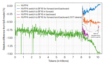
Importantly:
- The majority of the loss discrepancy could be attributed to the quantized forward pass, so switching to higher precision only for the
FPropcan help recovery while sustaining throughput. - Switching to higher precision during last ~18% of training can close the loss gap, and switching at even ~1% can result in significant recovery.
From a practical perspective, their recommendation is to switch to higher precision during the final cooldown (weight decay) phase of training.
Recipe Summary
| GEMM | RHT | Scaling | Rounding |
|---|---|---|---|
| Fprop | N | : 1D, : 2D | RTN |
| Dgrad | N | : 1D, : 2D | : SR |
| Wgrad | Y | : 1D, : 1D | : RTN, : SR |
Next: Part 2: Systems Optimizations — Systems optimizations and custom kernels for making NVFP4 performant.
References
Epoch AI. "Training Compute of Frontier AI Models Grows by 4.5x per Year." (2024).
DeepSeek-AI. "DeepSeek-V3 Technical Report." arXiv (2024).
Dan Fu. "AGI-scaling." (2025).
Open Compute Project. "OCP Microscaling Formats (MX) v1.0 Spec." (2023).
NVIDIA. "Blackwell Architecture." (2025).
NVIDIA. "Pretraining Large Language Models with NVFP4." arXiv (2025).
Cook et al. "Four Over Six: More Accurate NVFP4 Quantization with Adaptive Block Scaling." arXiv (2025).
Chen et al. "TetraJet-v2: Accurate NVFP4 Training for Large Language Models." arXiv (2025).
Castro et al. "Quartet: Native FP4 Training Can Be Optimal for Large Language Models." arXiv (2025).
NVIDIA. "Transformer Engine Documentation." (2024).
NVIDIA. "NVIDIA Debuts Nemotron-3 Family of Open Models." (2025).
NVIDIA. "Nemotron 3: Efficient and Open Intelligence." arXiv (2025).
NVIDIA. "GTC 2025: Blackwell Numerics for AI." (2025).
Micikevicius et al. "Mixed Precision Training." ICLR (2018).
Micikevicius et al. "FP8 Formats for Deep Learning." arXiv (2022).
NVIDIA. "Stable and Scalable FP8 Deep Learning." GTC (2025).
PyTorch. "Accelerating Large Scale Training with PyTorch Float8 Rowwise." (2025).
Meta. "Llama 3 Herd of Models." arXiv (2024).
Rouhani et al. "Microscaling Data Formats for Deep Learning." arXiv (2023).